Prediction in Multiple
Regression
Jason W. Osborne
University of Oklahoma
There are two general applications for multiple regression (MR): prediction
and explanation1. These roughly correspond to two differing goals in
research: being able to make valid projections concerning an outcome for a
particular individual (prediction), or attempting to understand a phenomenon by
examining a variable's correlates on a group level (explanation). There has been
debate as to whether these two applications of MR are grossly different, as
Scriven (1959) and Anderson and Shanteau, (1977) asserts, or necessarily part
and parcel of the same process (e.g., DeGroot, 1969, Kaplan, 1964; for an
overview of this discussion see Pedhazur, 1997, pp. 195-198). Regardless of the
philosophical issues, there are different analytic procedures involved with the
two types of analyses. The goal of this paper is to present: (a) the concept of
prediction via MR, (b) the assumptions underlying multiple regression analysis,
(c) shrinkage, cross-validation, and double cross-validation of prediction
equations, and (d) how to calculate confidence intervals around individual
predictions.
What is the Difference between Using MR
for Prediction versus Using MR for Explanation?
When one uses MR for explanatory purposes, that person is exploring
relationships between multiple variables in a sample to shed light on a
phenomenon, with a goal of generalizing this new understanding to a population.
When one uses MR for prediction, one is using a sample to create a regression
equation that would optimally predict a particular phenomenon within a
particular population. Here the goal is to use the equation to predict outcomes
for individuals not in the sample used in the analysis. Hypothetically,
researchers might create a regression equation to predict twelfth-grade
achievement test scores from eighth-grade variables, such as family
socioeconomic status, race, sex, educational plans, parental education, GPA, and
participation in school-based extracurricular activities. The goal is not to
understand why students achieve at a certain level, but to create the best
equation so that, for example, guidance counselors could predict future
achievement scores for their students, and (hopefully) intervene with those
students identified as at risk for poor performance, or to select students into
programs based on their projected scores. And while theory is useful for
identifying what variables should be in a prediction equation, the variables do
not necessarily need to make conceptual sense. If the single greatest predictor
of future achievement scores was the number of hamburgers a student eats, it
should be in the prediction equation regardless of whether it makes sense
(although this sort of finding might spur some explanatory research�.)
How is a Prediction Equation Created?
The general process for creating a prediction equation involves gathering
relevant data from a large, representative sample from the population. What
constitutes "large" is open to debate, and while guidelines for
general applications of regression are as small as 50 + 8*number of predictors (Tabachnick
& Fidell, 1996), guidelines for prediction equations are more stringent due
to the need to generalize beyond a given sample. While some authors have
suggested that 15 subjects per predictor is sufficient (Park & Dudycha,
1974; Pedhazur, 1997), others have suggested minimum total sample (e.g., 400,
see Pedhazur, 1997), others have suggested a minimum of 40 subjects per
predictor (Cohen and Cohen, 1983; Tabachnick & Fidell, 1996). Of course, as
the goal is a stable regression equation that is representative of the
population regression equation, more is better. If one has good estimates of
effect sizes, a power analysis might give a good estimate of the sample size.
The effect of sample size on shrinkage and stability will be explored below.
Methods for entering variables into the equation. There are many ways to
enter predictors into the regression equation. Several of these rely on the
statistical properties of the variables to determine order of entry (e.g.,
forward selection, backward elimination, stepwise). Others rely on the
experimenter to specify order of entry (hierarchical, blockwise), or have no
order of entry (simultaneous). Current practice clearly favors
analyst-controlled entry, and discourages entry based on the statistical
properties of the variables as it is atheoretical. A thorough discussion of this
issue is beyond the scope of this paper, so the reader is referred to Cohen and
Cohen (1983) and Pedhazur (1997) for overviews of the various techniques, and to
Thompson (1989) and Schafer (1991a, 1991b) for more detailed discussions of the
issues.
Regardless of the method ultimately chosen by the researcher, it is critical
that the researcher examine individual variables to ensure that only variables
contributing significantly to the variance accounted for by the regression
equation are included. Variables not accounting for significant portions of
variance should be deleted from the equation, and the equation should be
re-calculated. Further, researchers might want to examine excluded variables to
see if their entry would significantly improve prediction (a significant
increase in R-squared).
What Assumptions Must be Met When Doing
a Regression Analysis?
It is absolutely critical that researchers assess whether their analyses meet
the assumptions of multiple regression. These assumptions are explained in
detail in places such as Pedhazur (1997) and Cohen and Cohen (1983), and as such
will not be addressed further here. Failure to meet necessary assumptions can
cause problems with prediction equations, often serving to either make them less
generalizable than they otherwise would be, or causing underprediction
(accounting for less variance than they should, such as in the case of
curvilinearity or poor measurement).
How Are Prediction Equations Evaluated?
In a prediction analysis, the computer will produce
a regression equation that is optimized for the sample. Because this process
capitalizes on chance and error in the sample, the equation produced in one
sample will not generally fare as well in another sample (i.e., R-squared in
a subsequent sample using the same equation will not be as large as R-squared
from original sample), a phenomenon called shrinkage. The most desirable outcome
in this process is for minimal shrinkage, indicating that the prediction equation
will generalize well to new samples or individuals from the population examined.
While there are equations that can estimate shrinkage, the best way to estimate
shrinkage, and test the prediction equation is through cross-validation or double-cross
validation.
Cross-validation. To perform cross-validation,
a researcher will either gather two large samples, or one very large sample
which will be split into two samples via random selection procedures. The prediction
equation is created in the first sample. That equation is then used to create
predicted scores for the members of the second sample. The predicted scores
are then correlated with the observed scores on the dependent variable (ryy').
This is called the cross-validity coefficient. The difference between
the original R-squared and ryy'2 is the shrinkage.
The smaller the shrinkage, the more confidence we can have in the generalizability
of the equation.
In our example of predicting twelfth-grade achievement
test scores from eighth-grade variables a sample of 700 students (a subset of
the larger National Education Longitudinal Survey of 1988) were randomly split
into two groups. In the first group, analyses revealed that the following eighth-grade
variables were significant predictors of twelfth-grade achievement: GPA, parent
education level, race (white=0, nonwhite=1), and participation in school-based
extracurricular activities (no=0, yes=1), producing the following equation:
Y'= -2.45+1.83(GPA) -0.77(Race) +1.03(Participation)
+0.38(Parent Ed)
In the first group, this analyses produced an R-squared
of .55. This equation was used in the second group to create predicted scores,
and those predicted scores correlated ryy' = .73
with observed achievement scores. With a ryy'2
of .53 (cross-validity coefficient), shrinkage was 2%, a good outcome.
Double cross-validation. In double cross-validation prediction equations
are created in both samples, and then each is used to create predicted scores
and cross-validity coefficients in the other sample. This procedure involves
little work beyond cross-validation, and produces a more informative and
rigorous test of the generalizability of the regression equation(s).
Additionally, as two equations are produced, one can look at the stability of
the actual regression line equations.
The following regression equation emerged from analyses of the second
sample::
Y'= -4.03 +2.16(GPA) -1.90(Race) +1.43(Participation)
+0.28(Parent Ed)
This analysis produced an R-squared of .60. This equation was used in the
first group to create predicted scores in the first group, which correlated .73
with observed scores, for a cross-validity coefficient of .53. Note that: (a)
the second analysis revealed larger shrinkage than the first, (b) the two
cross-validation coefficients were identical (.53), and (c) the two regression
equations are markedly different, even though the samples had large subject to
predictor ratios (over 80:1).
How much shrinkage is too much shrinkage? There are no clear guidelines
concerning how to evaluate shrinkage, except the general agreement that less is
always better. But is 3% acceptable? What about 5%? 10%? Or should it be a
proportion of the original R-squared (so that 5% shrinkage on an R-squared of
.50 would be fine, but 5% shrinkage on an R-squared of .30 would not be)? There
are no guidelines in the literature. However, Pedhazur has suggested that one of
the advantages of double cross-validation is that one can compare the two
cross-validity coefficients, and if similar, one can be fairly confident in the
generalizability of the equation.
The final step. If you are satisfied with your shrinkage statistics, the
final step in this sort of analysis is to combine both samples (assuming
shrinkage is minimal) and create a final prediction equation based on the larger
sample. In our data set, the combined sample produced the following regression
line equation:
Y'= -3.23 +2.00(GPA) - 1.29(Race) +1.24(Participation) +0.32(Parent Ed)
How does sample size affect the
shrinkage and stability of a prediction equation?
As discussed above, there are many different opinions
as to the minimum sample size one should use in prediction research. As an illustration
of the effects of different subject to predictor ratios on shrinkage and stability
of a regression equation, data from the National Education Longitudinal Survey
of 1988 (NELS 88, from the National Center for Educational Statistics) were
used to construct prediction equations identical to our running example. This
data set contains data on 24,599 eighth grade students representing 1052 schools
in the United States. Further, the data can be weighted to exactly represent
the population, so an accurate population estimate can be obtained for comparison.
Two samples, each representing ratios of 5, 15, 40, 100, and 400 subjects per
predictor were randomly selected from this sample (randomly selecting from the
full sample for each new pair of a different size). Following selection of the
samples, prediction equations were calculated, and double cross-validation was
performed. The results are presented in Table 1.
Table 1: Comparison of double cross validation results
with differing
subject:predictor ratios
| Sample Ratio
(subjects: predictors)
|
Obtained Prediction Equation
|
R2
|
ryy'2
|
Shrink-
age
|
|
Population
|
Y'= -1.71+2.08(GPA) -0.73(race) -0.60(part) +0.32(pared)
|
.48
|
|
|
|
5:1
|
|
Sample 1
|
Y'= -8.47 +1.87(GPA) -0.32(race) +5.71(part) +0.28(pared)
|
.62
|
.53
|
.09
|
|
Sample 2
|
Y'= -6.92 +3.03(GPA) +0.34(race) +2.49 (part) -0.32(pared)
|
.81
|
.67
|
.14
|
|
15:1
|
|
Sample 1
|
Y'= -4.46 +2.62(GPA) -0.31(race) +0.30(part) +0.32(pared)
|
.69
|
.24
|
.45
|
|
Sample 2
|
Y'= -1.99 +1.55(GPA) +0.34(race) +1.04 (part) -0.58(pared)
|
.53
|
.49
|
.04
|
|
40:1
|
|
Sample 1
|
Y'= -0.49 +2.34(GPA) -0.79(race) -1.51(part) +0.08(pared)
|
.55
|
.50
|
.05
|
|
Sample 2
|
Y'= -2.05 +2.03(GPA) -0.61(race) -0.37(part) -+0.51(pared)
|
.58
|
.53
|
.05
|
|
100:1
|
|
Sample 1
|
Y'= -1.89 +2.05(GPA) -0.52(race) -0.17(part) +0.35(pared)
|
.46
|
.45
|
.01
|
|
Sample 2
|
Y'= -2.04 +1.92(GPA) -0.01(race) +0.32(part) +0.37(pared)
|
.46
|
.45
|
.01
|
|
400:1
|
|
Sample 1
|
Y'= -1.26 +1.95(GPA) -0.70(race) -0.41(part) +0.37(pared)
|
.47
|
.46
|
.01
|
|
Sample 2
|
Y'= -1.10 +1.94(GPA) -0.45(race) -0.56(part) +0.35(pared)
|
.42
|
.41
|
.01
|
The first observation from the table is that, by
comparing regression line equations, the very small samples have wildly fluctuating
equations (both intercept and regression coefficients). Even the 40:1 ratio
samples have impressive fluctuations in the actual equation. While the fluctuations
in the 100:1 sample are fairly small in magnitude, some coefficients reverse
direction, or are far off of the population regression line. As expected, it
is only in the largest ratios presented, the 100:1 and 400:1 ratios, that the
equations stabilize and remain close to the population equation.
Comparing variance accounted for, variance accounted
for is overestimated in the equations with less than a 100:1 ratio. Cross-validity
coefficients vary a great deal across samples until a 40:1 ratio is reached,
where they appear to stabilize. Finally, it appears that shrinkage appears to
minimize as a 40:1 ratio is reached. If one takes Pedhazur's suggestion to compare
cross-validity coefficients to determine if your equation is stable, from these
data one would need a 40:1 ratio or better before that criterion would be reached.
If the goal is to get an accurate, stable estimate of the population regression
equation (which it should be if that equation is going to be widely used outside
the original sample), it appears desirable to have at least 100 subjects per
predictor.
Calculating a Predicted Score, and
Confidence Intervals Around That Score
There are two categories of predicted scores relevant
here: scores predicted for the original sample, and scores that can be predicted
for individuals outside the original sample. Individual predicted scores and
confidence intervals for the original sample are available in the output available
from most common statistical packages. Thus, the latter will be addressed here.
Once an analysis is completed and the final regression line equation is
formed, it is possible to create predictions for individuals who were not part
of the original sample that generated the regression line (one of the attractive
features of regression). Calculating a new score based on an existing regression
line is a simple matter of substitution and algebra. However, no such prediction
should be presented without confidence intervals. The only practical way to do
this is through the following formula:
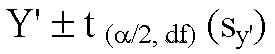
where sy' is calculated as: 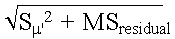
where  is the squared standard error of mean predicted scores (standard error of the
estimate, squared), and the mean square residual, both of which can be obtained
from typical regression output.2
is the squared standard error of mean predicted scores (standard error of the
estimate, squared), and the mean square residual, both of which can be obtained
from typical regression output.2
Summary and suggestions for further study
Multiple regression can be an effective tool for
creating prediction equations providing adequate measurement, large enough samples,
assumptions of MR are met, and care is taken to evaluate the regression equations
for generalizability (shrinkage). Researchers interested in this topic might
want to explore the following topics: (a) the use of logistic regression for
predicting binomial or discrete outcomes, (b) the use of estimation procedures
other than ordinary least squares regression that can produce better prediction
(e.g., Bayesian estimation, see e.g. Bryk and Raudenbush, 1992), and (c) alternatives
to MR when assumptions are not met, or when sample sizes are inadequate to produce
stable estimates, such as ridge regression (for an introduction to these alternative
procedures see e.g., Cohen & Cohen, 1983, pp.113-115). Finally, if researchers
have nested or multilevel data, they should use multilevel modeling procedures
(e.g., HLM, see Bryk & Raudenbush, 1992) to produce prediction equations.
SUGGESTED READING:
Anderson, N. H., & Shanteau, J. (1977). Weak inference
with linear models. Psychological Bulletin, 84, 1155-1170.
Bryk, A.S., & Raudenbush, S. W. (1992). Hierarchical
linear models: Applications and data analysis methods. Newbury Park, CA:
Sage Publications.
Cohen, J., & Cohen, P. (1983). Applied multiple
regression/correlation analysis for the behavioral sciences. Hillsdale, NJ:
Lawrence Erlbaum Associates, Inc.
DeGroot, A. D. (1969). Methodology: Foundations of
inference and research in the behavioral sciences. The Hague: Mouton.
Kaplan, A. (1964). The conduct of inquiry: Methodology for
behavioral science. San Francisco: Chandler.
Park, C., & Dudycha, A. (1974). A cross-validation
approach to sample size determination. Journal of the American Statistical
Association, 69, 214-218.
Pedhazur, E. J. (1997). Multiple
regression in behavioral research. Harcourt Brace: Orlando, FL.
Scriven, M. (1959). Explanation and prediction in evolutionary theory. Science,
130, 477-482.
Thompson, B. (1989). Why won't stepwise methods die? Measurement and
Evaluation in Counseling and Development, 21, 146-148.
Schafer, W. D. (1991a). Reporting hierarchical regression results. Measurement
and Evaluation in Counseling and Development, 24, 98-100.
Schafer, W.D. (1991b). Reporting nonhierarchical regression results. Measurement
and Evaluation in Counseling and Development, 24, 146-149.
Tabachnick, B. G., & Fidell, L. S. (1996). Using Multivariate
Statistics. New York: Harper Collins.
FOOTNOTES
1. Some readers may be uncomfortable with the term
"explanation" when referring to multiple regression, as these data
are often correlational in nature, while the term explanation often implies
causal inference. However, explanation will be used in this article because:
(a) it is the convention in the field, (b) here we are talking of regression
with the goal of explanation, and (c) one can come to understanding of
phenomena by understanding associations without positing or testing strict causal
orderings..
2. It is often the case that one will want to use standard error of the
predicted score when calculating an individual confidence interval. However, as
that statistic is only available from statistical program output, and only for
individuals in the original data set, it is of limited value for this
discussion. Here we suggest using the standard error of the mean predicted
scores, as it is the best estimate of the standard error of the predicted score,
knowing it is not completely ideal, but lacking any other alternative.
AUTHOR NOTES
Correspondence relating to this article can be addressed to Jason W. Osborne,
Department of Educational Psychology, University of Oklahoma, 820 Van Vleet
Oval, Norman, OK, 73019, or via email at josborne@ou.edu. Special thanks go to
William Schafer, whose many good suggestions and critical eye helped to
substantially shape this paper.
Sitemap 1 - Sitemap 2 - Sitemap 3 - Sitemap 4 - Sitemape 5 - Sitemap 6
