Exploratory
Longitudinal Profile Analysis via Multidimensional Scaling
Cody Ding
University of Missouri - St. Louis
Studying change processes in education and the
behavioral sciences has been of interest for a long time.Ā Researchers and
practitioners in the behavioral sciences are concerned with questions about how
individuals change over time (Willett & Sayer, 1994; Williamson, Appelbaum,
& Epanchin, 1991).Ā That is, we are interested in the question of how
individual change in certain attributes (for example, change of masculinity and
femininity among adolescents) is related to selected characteristics of a
person's background, family and peer environment, or training.Ā In recent
years, the number of models utilized to address questions of this kind has
increased substantially (e.g., Collins & Horn, 1991; Aber & McArdle,
1991).Ā
The focus of this paper is not to
compare different methods in modeling growth curve. Rather, the current study
is to propose a longitudinal profile analysis via Multidimensional Scaling
(PAMS), called LPAMS model.Ā This is an exploratory approach to identify growth
patterns in the data using Multidimensional Scaling, an alternative to more
commonly used theory-based structural equations model approach (e.g., McArdle
& Epstein, 1987).Ā
The longitudinal
multidimensional scaling analysis described here is an exploratory technique.Ā
There are several reasons for using the LPAMS model rather than more
traditional approaches such as structural equations modeling.Ā First, the LPAMS
model is most suitable for the situation in which the growth patterns are to be
derived from the data, rather than specified by theory.Ā It requires no a
priori hypotheses about the nature of the underlying growth patterns.Ā While a
priori specification of a unidimensional growth pattern model is often
feasible, the difficulty of specifying the growth patterns a priori increases
as the number of growth curves increases.
Second, it provides
estimates of latent growth pattern as well as estimates of individual growth
parameters in the model (that is, growth rate estimates for each individuals),
not simply summary statistics such as means, variances, and covariances.Ā If
one wishes to study inter-individual differences in growth profiles, one may
take the individual growth parameter estimates as a description of his or her
entire growth pattern and subject those parameter estimates to multivariate
analysis of variance or regression analysis.Ā
In a sense, LPAMS is
similar to multilevel or hierarchical modeling in that it allows one to
estimate both group level growth parameters and individual growth rate, where
within-subject is considered level 1 model and between-subjects is considered
level 2 model (Willett & Sayer, 1994).Ā After obtaining level 1 individual
growth rate estimate and initial status estimate, one can examine between-group
differences in these parameter estimates.Ā The differences between the LPAMS
model and the commonly-used hierarchical linear model (HLM) are that: First, in
HLM there is clustering of individuals within group and variables are measured
at all available levels, thus combining variables from different levels in one
statistical model, whereas in the LPAMS model one estimates within-individual
change with respect to the latent change curves using MDS method and estimates
between-individual variations via conventional ANOVA approach.Ā Second, they
differ on some of the assumptions, which are discussed below.
Third, the assumptions
are minimal.Ā The more traditional models suffer from complaints about the theoretical
restrictions and lack of applicability of many standard linear models that
assume the normal distribution (Nesselroade & Ford, 1987; Nesselroad &
Cattell, 1989).Ā The LPAMS model allows for simultaneous estimation intra- and
inter-individual growth processes without requirement of the multivariate
normality of tests frequently employed.Ā It can be applied to the data that are
not amenable to the common methods of analysis due to limitations imposed by
the specific design of experiment, or theoretical assumptions about the nature
of the phenomenon under study.Ā
Fourth, the LPAMS model
is based on distance model (Borg & Groenen, 1997; Davison, 1983) rather
than linear model.Ā Thus, it can be used to model data that are nonlinear in
nature.Ā In LPAMS modeling, the growth patterns are examined, not just mean
score change over time, which can usually be analyzed using a standard
univariate or multivariate repeated-measures design.Ā This is especially the
case when there may be more than one growth curves in the data and the LPAMS
model can simultaneously identify these curves.ĀĀĀĀĀ
As with any methodology, there are several
limitations associated with this exploratory longitudinal MDS approach.Ā First,
as with any exploratory approach, it is designed to identify patterns of growth
underlying a set of data, not to test a priori hypotheses about patterns.Ā
Therefore, it will often be most useful in the early stages of a research
program in which little is known about the underlying growth patterns.Ā Second,
while it requires no distributional assumptions about the observed variables,
it does require equal error variances at each time period, which may not be
realistic.Ā
In rest of the paper, the focus will be on
discussing the multidimensional scaling (MDS) model underlying longitudinal
profile analysis and on how the LPAMS model can be used for growth curve
analysis.Ā Next, parameter estimation is considered.Ā The parameter estimation
scheme involves obtaining an initial estimate of growth curve parameters,
re-scaling them to facilitate interpretation in the context of growth curve
analysis, and then estimating the individual growth parameters.
Longitudinal Profile
Analysis via Multidimensional Scaling (LPAMS)
Longitudinal Profile Analysis via MDS Model
A multidimensional
scaling (MDS) model produces a geometric or spatial representation of
relationships between stimuli or individuals.Ā The goal is to produce a
geometric representation of underlying individual or stimuli dimensions that
fit the data based on spatial proximity between pairs of objects as a measure
of their relatedness.Ā A classical MDS example used to identify latent stimuli
dimensions is the research on the childrenÆs cognitive reasoning of body parts
(Jacobowitz, 1975).Ā In this study, children were presented with pairs of body
parts.Ā They were asked to sort the body parts according to the functions of
these parts.Ā MDS was used to model the nature of a childÆs conception in the
geometric space in which subjects locate their perceptions of the different
body parts.ĀĀ
This geometric representation of
underlying stimuli can be extended to examining how a set of variables is
patterned or configured in a space.Ā The research focus is on what typical
patterns or configurations of variables actually exist in the population and
how individuals differ with respect to these patterns.Ā This is what MDS
profile analysis attempts to answer (e.g., Davison, Gasser, & Ding, 1996;
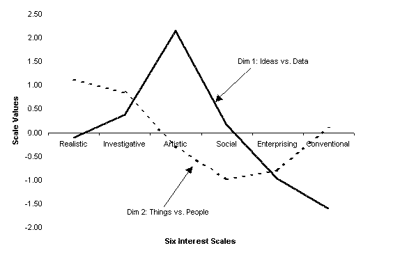
Davison, Kuang, & Kim, 1999).Ā Figure 1 is an example of such a latent
profile analysis of vocational interest profiles based on well-known hexagonal
theory of vocational interest (Campbell & Hansen, 1985).ĀĀ As can be seen
from the figure, each interest variable is located along the two dimensions
according to their scale values xk(t), which quantify the
relationships among the variables under inquiry.
| Figure 1.Ā Latent profile patterns for vocational
interests. |
 |
The above examples serve to
demonstrate two applications of the MDS model.Ā One can build on these concepts
and extend the model for longitudinal studies.Ā When the variable under the
study is repeated at different occasions, however, the repeated variable is
expected to be related to one other in the form of a particular developmental
shape along the certain dimensions.Ā Therefore, one may conceptualize the
magnitude of that variable as a function of characteristics of that person as
well as time of measurement.Ā The MDS model used in such longitudinal data
analysis is called longitudinal profile analysis via multidimensional scaling
(LPAMS) model.Ā In this model, each growth curve dimension k represents
an exemplar of a particular arrangement of scores of different time points,
called a prototypical growth pattern or latent growth pattern, which is defined
by the scale value xk(t) estimates from the model.Ā
Longitudinal profile
analysis via MDS model starts with the equation:
| m p(t)
= Sk wpk xk(t)
+ cp + ep(t) |
(1) |
where m p(t) is the score of person p
at time t; xk(t) is scale value estimates that reflect
the location of a repeated variable at time t along the developmental
curve k, leading to kth unspecified longitudinal curve
for all individuals; wpk is an individual growth profile
index that the person p attaches to the xk(t),
quantifying the degree to which each individualÆs observed profiles resemble
the several dimensions (patterns) indexed by the subscript k.Ā Each
dimension k can be considered a growth trajectory, and each personÆs
individual growth profile is modeled as a linear combination of the K
trajectories represented by dimensions; cp is a level
parameter or intercept estimate, and ep(t) is an error term.
The point of the foregoing
discussion is that a set of variables or a set of scores of a repeated variable
can be configured in a multidimensional space according to their locations in
k-spaces; a particular arrangement of scores based on their scale value
estimates may form a latent pattern or growth curve.Ā This pattern does not
indicate homogeneity of construct of a set of variables, as in factor analysis;
rather it represents a psychological characteristic shape and level of the
variable under inquiry.ĀĀĀĀĀ
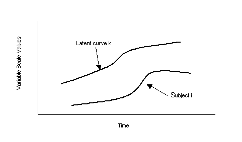
Graphically the concepts of kth
latent growth shape and an individual growth profile can be represented as that
in Figure 2.
| Figure 2.Ā The kth latent growth shape
and an individual growth pattern. |
 |
The intercept or level parameter, cp,
can be defined in several ways, depending on how the origin of the MDS solution
is set.Ā In longitudinal data analysis, for example, if one wishes to study
growth curve, the zero point can be set to correspond with the scale value at
the first time period (i.e., xk(1) = 0 for all k),
then cp becomes the expected score under the model for person
p at the initial time t = 1.Ā That is, in Equation 1, if xk(1)
= 0 for every k, then the model predicted data point at time 1 for
person p, mp(1)ó
= Sk wpk xk(1)
+ cp Āreduces to mp(1)ó = cp.Ā Given the
importance of initial level in the literature on growth, researchers may wish
to set the zero point along dimensions so that the intercept for person p
can be interpreted as the model predicted estimate of initial level for person p.Ā
Estimating Parameters in the Model.ĀĀĀĀĀĀĀĀĀ
The LPAMS model analysis begins by
using MDS to obtain initial estimates of the scale values xk(t)
in the model of Equation 1.Ā Once the initial estimates are obtained, the zero
point on each dimension can be re-scaled so that intercept or level parameter
estimate can be interpreted as initial level.Ā Having set the origin of
dimensions, the individual growth parameters in the model, cp
and wpk, can then be estimated by regressing the raw data mp(t)
in row p onto the now-known scale value estimates, xk(t).Ā
AssumptionsĀĀ LPAMS analysis
model is based on distance model.Ā The assumptions on which the LPAMS analysis
is based are mostly restrictions to uniquely identify the MDS solution rather
than assumptions that limit the fit of the model to the data.Ā The only
assumptions of Equation 1 are that (1) the variance of the deviations about the
model be equal at all occasions of measurement, i.e., (1/P)Σep(t)2
= σ2(e) for all t and (2) the errors are
independently distributed with mean zero.Ā Beyond these, the analysis requires
no other distributional assumptions such as normality.ĀĀ
Initial MDS Estimates of Scale Value xk(t).Ā
In an LPAMS analysis based on distance model, the analysis begins with a matrix
containing a proximity measure defined over all possible pairs of stimuli.Ā In
fact, the choice between using a distance measure and a correlation/covariance
is not that important (Borg & Groenen, 1997).Ā In our case, the stimuli are
time points, and the proximity measure for each possible pair of time points (t,
tÆ) is a squared Euclidean distance measure, dtt'2, computed from the raw data as
follows:
| dtt'2
= (1/P)Sp(mp(t) -
mp(tÆ))2 |
(2) |
Table 1 shows the square root of squared Euclidean distance
matrix thus computed based on reading achievement.Ā The distance coefficients
indicates the degree to which the reading scores differ from each other over
time.Ā The proximity module in many standard statistical packages (e.g. SAS,
SPSS, SYSTAT) includes an option for the computation of squared Euclidean
distance or Euclidean distance proximity measures defined over all possible
pairs of variables.Ā
|
Table 1: Euclidean Distance Matrix of the Reading Scores Over Four
Occasions
|
|
|
1997
|
1998
|
1999
|
2000
|
|
1997
|
0
|
449.72
|
768.22
|
893.33
|
|
1998
|
713.32
|
0
|
583.85
|
693.33
|
|
1999
|
867.25
|
427.34
|
0
|
388.75
|
|
2000
|
1076.33
|
581.75
|
420.63
|
0
|
|
Note.Ā Numbers above
diagonal are for grade 5 cohort and numbers below diagonal are for grade 3 cohort. |
When proximity measures Equation 2 are submitted
to an appropriate multidimensional scaling algorithm, the analysis should yield
one dimension for each latent growth curve.Ā Since the objective of the LPAMS
model analysis is to see if there are particular trend shapes in the data,
whether they are linear curve, nonlinear curve, or time-series periodic curves,
MDS estimation method would identify one or more such trend shapes when such
curves exist in the data.Ā Thus, LPAMS model configures repeated data points in
k-dimensions, and the scale value for time t along dimension k
will provide an estimate of xk(t) in the LPAMS model of
Equation 1, with these estimates representing the prototypical growth patterns
along the dimensions.Ā ĀĀĀ
Re-scaling the Origin of the
Dimensions.ĀĀ In most, if not all, MDS algorithms, the zero point along
each dimension is set equal to the mean scale value along that dimension.Ā
Consequently, if one employs commonly available MDS algorithms, the zero point
along each dimension may not be set so as to yield the desired interpretation
of the intercept parameter cp.Ā After x*k(t),
the initial estimate of the scale value for time t along dimension k,
is obtained, the zero point can be re-set so as to correspond with the location
of the first time period simply by taking each initial estimate and subtracting
x*k(1).Ā That is, the final estimate of each scale value xk(t)
can be computed from the initial estimates according to the following formula: xk(t)
= Āx*k(t) ¢ x*k(1) for all k
and t.Ā If the origin is thus re-set, each intercept parameter estimate
(obtained below) can be interpreted as the initial level for person p.Ā
Such change of the origin must take place before estimating the person
parameters in the next step in order to obtain the desired interpretation of
the intercept estimates.
Estimating Individual
Differences Parameters.Ā Once the final scale values have been obtained,
least squares estimates of the person parameters, cp and wpk,
can be estimated through regression.Ā By treating mp(t) as scores
on a ōcriterionö variable and the scale values along each dimension as
ōpredictorö scores, one can regress the criterion variable, the data mp(t)
in row p, onto the several predictor dimensions, xk(t),
to estimate the intercept cp and the several growth profile
index (also called slope or salience weight) wpk for person p.Ā
Thus, LPAMS model analysis proceeds in three
steps.Ā First, proximity measures are computed over all possible pairs of times
according to Equation 2.Ā These proximity measures are analyzed using nonmetric
MDS algorithms to yield estimates of the scale values xk(t)
in theĀ model.Ā In the second step, the zero point along each dimension is
re-set, if necessary, so that the estimates of the intercept parameters will
have the desired interpretation.Ā Finally, the individual growth parameters cp
and wpk are estimated by regressing each personÆs raw data
onto the MDS scale values.Ā
A concrete example may elucidate the LPAMS model
analysis.Ā The SAS codes are provided in the appendix so that reader can carry
out the analysis.Ā The data were from student reading achievement over a
four-year span.Ā Like many in the literature, it includes only one latent
growth pattern, i.e., only one dimension.Ā It should be noted that this was a
coincident in that there were only four repeated measures available over four
years for the current study.Ā In fact, more data points are desirable in such
applications so that different growth curves can be studied.ĀĀĀ
LPAMS Growth Profile
Analysis on Reading Achievement Test
To illustrate the use of the LPAMS
model for exploratory growth profile analysis, a data set containing four waves
of data was used.Ā The data was obtained from a sample of 705 elementary and
middle school students at a school district in a Southwest state.Ā These
students consisted of 2 cohorts.Ā Grade 3 cohort students were in 3rd
grade at the first time of measurement and grade 5 cohort students were in 5th
grade at the first time of testing.Ā The same students were followed for four
years.Ā For grade 3 cohort, each students completed the Stanford Reading
Test---Ninth edition at each grade (i.e., at 3rd, 4th, 5th,
and 6th grades).Ā Similarly, grade 5 cohort students were repeatedly
assessed using the same test at 5th, 6th, 7th,
and 8th grade.Ā The test was used by the school district to measure
students' academic progress over the years.Ā The scores were reported as scaled
scores for each student across these four waves of data collection.Ā
Table 2 shows the means and
standard deviations of the reading scores for these two cohorts.Ā These
statistics are based on 705 students who had complete data on all four
occasions of measurement.Ā Inspection of the table indicated that students did
seem to progress in their reading achievement over the years, with grade 3
cohort students showing decreased variations over time, indicating on average
students were less scattered in their reading scores.Ā
|
Table 2: Means and Standard Deviations For the Reading Scores at Four
Occasions
|
|
|
Grade 3 Cohort
(n=333)
|
Grade 5 Cohort
(n=372)
|
|
Reading 97
|
615.18 (37.97)
|
656.03 (33.02)
|
|
Reading 98
|
645.98 (36.24)
|
667.24 (28.96)
|
|
Reading 99
|
656.59 (33.32)
|
688.93 (34.34)
|
|
Reading 00
|
668.71 (30.87)
|
697.32 (30.80)
|
|
Note.Ā Numbers in parenthesis are standard deviations. |
Exploratory LPAMS Analysis of Growth Profiles
Exploratory longitudinal profile
analysis via multidimensional scaling (LPAMS) started with estimating scale
values presented in Equation 1.Ā As mentioned above, time is specified as the
latent dimension along which individuals vary with regard to the growth/decline
curve.Ā In applying this model, the reading score is considered a repeatedly
measured variable on a time dimension along which individual change patterns
are of interest.Ā Since the analysis is exploratory, no specification of a
particular growth/decline profile is necessary.Ā The growth patterns are to be
derived from the observed data.
Estimating scale valuesĀĀ In
the LPAMS growth analysis, the squared Euclidean distance was first computed
from raw scores on reading tests based on Equation 2, which were then used as
input for nonmetric MDS analysis using SAS.
Next, initial scale values, xk(t),Ā
were estimated using nonmetric MDS procedures and one dimensional solution was
identified.Ā These scale values reflect growth rates over a four year span.Ā As
a rule, five or more variables are needed to define a dimension (Davison,
1983).Ā Since there were only four repeatedly measured variables in the current
data, no more than one trajectory dimension (i.e., one growth pattern) seemed
to be justified.Ā The adequacy of a one dimensional MDS solution was verified
by the MDS fit index, STRESS-1 formula (Kruskal, 1964).Ā The STRESS-1 value was
zero (S1 = 0.00), indicating that the observed data points fit the
one-dimensional MDS model well.Ā
The estimates of LPAMS growth curve
values (i.e., scale values of the repeated variable) are presented in Table 3.Ā
The scale values in Table 3 are the final estimates obtained by re-scaling the
initial estimates in such a way that the zero point corresponds to the scale
value of time 1 so that intercept or level estimate indicate the initial
level.Ā To facilitate the presentation of the scale values, they were scaled to
have a mean of 5 and a standard deviation of 2.Ā This was a simple linear
transformation that did not affect the interpretation of the scale values.Ā
Growth rates in percentage for each of the three time intervals were also shown
in the table.Ā These growth rates remained the same regardless of the
translation of the scale values.
|
Table 3: Final Re-scaled Estimates of Scale Values for Reading
Achievement Over Four Year Span
|
|
|
|
Scaled Scale Values
|
|
|
Grade 3 Cohort
|
Grade 5 Cohort
|
|
Reading 97
|
1.82 (0%)
|
2.38 (0%)
|
|
Reading 98
|
4.94 (58%)
|
3.80 (29%)
|
|
Reading 99
|
6.06 (79%)
|
6.48 (83%)
|
|
Reading 00
|
7.18 (100%)
|
7.34 (100%)
|
|
Note:Ā Percentages in parenthesis indicate the growth
rate in adjacent years. |
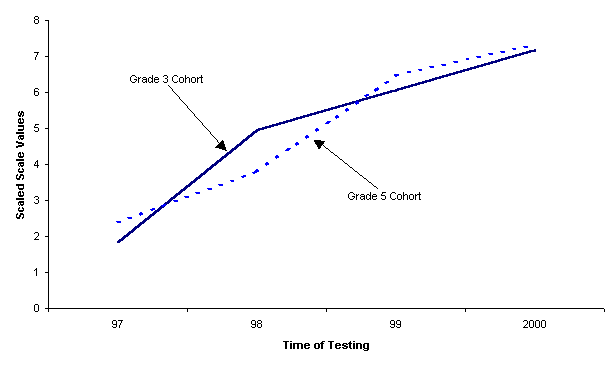
Figure 3 shows the latent growth
pattern based on the final growth scale values.Ā The dimension scale values
depict the latent growth pattern in terms of three line segments.Ā Each segment
covers one time interval: year 97 to 98, year 98 to 99, and year 99 to 2000.Ā
Differences in growth rate over the several time intervals are represented by
the slopes of the line segments for those intervals.ĀĀ As can be seen in Figure
3, for grade 3 cohort, the pattern showed the greatest growth rate from 3rd
grade to 4th grade.Ā In this pattern, 58% of the growth occurred
over this first interval.Ā The growth rate slowed down from 4th
grade to 6th grade.Ā In this pattern, 21% of the growth occurred
from 4th to 5th grade and 21% from 5th to 6th
grade.Ā For grade 5 cohort, the growth rate showed the slow growth rate from 5th
grade to 6th grade, with 29% of growth occurring over this first
interval.Ā The greatest growth rate occurred from 6th to 7th
grade.Ā In this pattern, 54% growth occurred.Ā In the last time interval,
growth rate slowed down again, with 17% growth in reading achievement.
| Figure 3.ĀĀ Latent growth pattern in reading achievement. |
 |
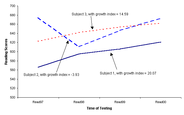
Estimating
individual growth parametersĀĀ The last step in the LPAMS growth profile
analysis was to estimate individual growth parameters cp and wpk
through regression.Ā cp is the intercept for person p,
and it can be interpreted as the model predicted estimate of initial level for
person p;Ā that is,Ā cp becomes the expected score
under the model for person p at the initial time (t = 1).Ā The wpk
are the growth profile index, quantifying the pthĀ individual
with regard to the kth ĀĀlatent
growth pattern and mapping the observed data onto growth trajectory represented
by the dimension.Ā If the model fits the data, then for any given interval,
growth is fastest for individuals with higher values of wpk.Ā
In Figure 4, subject 1 had a larger growth profile index than (w = 20.07) did
subject 3 (w = 14.59), with subject 1 showing faster growth than subject 3,
although both subjects resembled the latent growth profile.Ā Subject 2 had
slowest growth (-3.93) over time.
| Figure 4.ĀĀ Individual growth curve in reading
achievement. |
 |
In the current
data, the average of the growth profile index was 19.85, with a standard
deviation of 9.01 for grade 3 cohort, and was 16.50, with a standard deviation
of 8.08 for grade 5 cohort.Ā This indicated that, on average, students had made
gains in reading scores over the years, with certain individual variation in
growth profiles.Ā The correlation between the intercept cp
(i.e., initial status) and the profile correspondence index wpk
was -.59 and -.29 for each cohort respectively, indicating that students who
had high initial reading scores tended to make less gain in achievement over
the four year period.Ā
Conclusion
In recent years, latent growth curve modeling has
been widely used in longitudinal research.Ā Some authors (e.g., McArdle &
Epstein, 1987; Meredith & Tisak, 1990; Muthen, 1991) have demonstrated how
concepts of individual growth modeling can be accommodated within the framework
of covariance structure analysis.Ā In this paper, an exploratory growth profile
analysis was proposed.Ā The approach uses MDS model based on squared Euclidean
distance measures of proximity defined over pairs of time periods to model
growth curve in the data.Ā Such longitudinal profile analysis by means of MDS
can be used to study individual and group patterns of longitudinal change in an
exploratory fashion.Ā Latent growth rates are reflected in the estimates of
scale values from MDS geometric solutions, which could simultaneously
accommodate one or more growth curves in the data.Ā Individual growth profile
index is also estimated from the model so that one could directly study the
inter-individual differences with respect to growth.
One drawback of the current study is that there
are only 4 longitudinal data points available due to the difficult of obtaining
the longitudinal data with more time points.Ā This limits the demonstration of
using the LPAMS model to identify different growth curves in the data, which is
one of the major insights that can be made from the analysis.Ā Readers are
encouraged to try out this technique using their own data, preferably with
eight or more time points.
References
Aber, M. S.,
& McArdle, J. J.Ā (1991).Ā Latent growth curve approach to modeling the
development of competence.Ā In M. Chandler & M. Chapman (Eds.), Criteria
for competence: Controversies in the conceptualization and assessment of
children's abilities (pp. 231-258).Ā Mahwah, NJ: Lawrence Erlbaum
Associates.
Borg, I, &
Groenen, P.Ā (1997).Ā Modern Multidimensional Scaling:Ā Theory and applications.Ā
New York: Springer.
Campbell, D. P.,
& Hansen, J. C.Ā (1985).Ā Strong-Campbell Interest Inventory.Ā Palo
Alto, Stanford University Press.
Collins, L. M.,
& Horn, J. L.Ā (1991). Best methods for the analysis of change:Ā Recent
advance, unanswered questions, future directions.Ā Washington, DC:Ā
American Psychological Association.
Davison, M. L.,
Gasser, M., & Ding, S. (1996).Ā Identifying major profile patterns in a
population: An exploratory study of WAIS and GATB patterns.Ā Psychological
Assessment, 8, 26 ¢ 31.
Davison, M. L.,
Kuang, H., & Kim, S.Ā (1999).Ā The structure of ability profile patterns: A
multidimensional scaling perspective on the structure of intellect.Ā In P. L.
Ackerman, P. C. Kyllonen, & R.D. Roberts (Eds.).Ā Learning and
individual differences: Process, trait, and content determinants (pp. 187 ¢
204).Ā Washington, D. C.: APA Books.
Kruskal, J. B.Ā (1964).
Multidimensional scaling by optimizing goodness of fit to a nonmetric
hypothesis.Ā Psychometrika, 29, 1-27.
Jacobowitz, D.Ā
(1975).Ā The acquisition of semantic structures.Ā Unpublished doctoral
dissertation, University of North Carolina at Chapel Hill.
McArdle, J. J.,
& Epstein, D.Ā (1987).Ā Latent growth curves within developmental
structural equation models.Ā Child Development, 58, 110-133.
Meredith, W.,Ā & Tisak, J.Ā (1990).Ā Latent curve
analysis.Ā Psychometrika, 55, 107-122.
Muthen, B. O.Ā
(1991).Ā Analysis of longitudinal data using latent variable models with
varying parameters.Ā InĀ L. M. Collins & J. L. Horn (Eds.), Best methods
for the analysis of change:Ā Recent advance, unanswered questions, future
directions.Ā Washington, DC:Ā American Psychological Association.
Nesselroade, J. R.,
& Cattell, R. B.Ā (1989).Ā Handbook of multivariate experimental
psychology.Ā New York: Plenum Press.
Nesselroade, J.
R., & Ford, D.Ā (1987).Ā Putting the framework to work: Methodological
implications of the systems framework.Ā In D. Ford (Ed.), Human as
self-constructing living systems: a developmental perspective on
behavior and personality (pp. 47-79).Ā Hillsdale, NJ: Lawrence Erlbaum.
Willett, J. B.,
& Sayer, A. G.Ā (1994).Ā Using covariance structure analysis to detect
correlates and predictors of individual change over time.Ā Psychological
Bulletin, 116, 363-381.
Williamson, G.
L., Appelbaum, M., & Epanchin, A.Ā (1991).Ā Longitudinal analyses of
academic achievement.Ā Journal of Educational Measurement, 28, 61-76.
Appendix:Ā SAS Codes for Performing the LPAMS Analysis
%MACRO
GROWTH (data =, var =, dim =, dimname= , pout= , subid = );
DATA
trsf1 (Keep=&var);
set
&data;
ĀĀ
PROC
TRANSPOSE DATA=trsf1 OUT=out;
var
&var;
RUN;
%INCLUDEĀ
'C:\program files\SAS institute\sas\v8\STAT\SAMPLE\xmacro.SAS';
%INCLUDEĀ
'C:\program files\SAS institute\sas\v8\STAT\SAMPLE\DISTnew.SAS';
%INCLUDEĀ
'C:\program files\SAS institute\sas\v8\STAT\SAMPLE\stdize.SAS';
%DISTANCE
( DATA=out, METHOD=EUCLID, id=_name_, OUT=dis );
RUN;
PROC
PRINT data=dis; RUN;
/*MDS
analysis*/
PROC
MDS DATA=dis CONDITION=matrixĀ SHAPE=TriangleĀ LEVEL=ordinal
ĀĀĀĀ
COEF=iĀ FORMULA=1Ā FIT=1Ā DIMENSION= &dimĀ PFINAL
ĀĀĀĀ
OUT=scale_valueĀ OUTRES=cordres
ĀĀĀĀ
;
TITLE
"Nonmetric MDS Growth Scale Values";
TITLE
æĀĀ æ;
RUN;
/*Re-scale
and Estimate C and W*/
DATA
profile (KEEP= &dimname);
SET
scale_value (FIRSTOBS=2 );Ā
PROC
PRINT data=profile;
run;
PROC
IML;
USE
&data VAR{&var}; /*use original raw score variables*/
READ
all INTO M ;
USE
profile VAR{&dimname}; /*Read in initial scale values*/
READ
ALL INTO X;
X
= (X - X[1,1])* -1;
Ā
/*Re-set the origin of the initial scale value and make them all positive */
Print
X;
Print
"This is final re-scaled estimates of growth scale values";
/*computes
the weights and level parameters */
START
w;
R=NROW(x);
COL=J(r,1,1);
X1=X||COL;
M1=inv(X1`*X1);ĀĀ
M2=M*X1;
TW=M2*M1;
FINISH
W;
RUN
w;
/*computes
the fit measure for each subject*/
START
fit;
M1
= tw * x1`;
K
= ncol(m);
R
= nrow(m);
COL = j(1,k,1);
M1RSUM
= m1-((m1[,+]*col)/k );
PVAR
= (m1rsum##2)*col`;
MRSUM
= m - ((m[,+] * col)/k);
VAR
= (mrsum##2)*col`;
COL= pvar/var;
FINISH
fit;
run
fit;
/*Merge
weights and level parameters with the fit measures */
WL=tw||col;
/*Get
subject id from original data for merging dataset*/
use
&data Var{&subid};
read
all into id;
WL
= id||WL;
MATTRIB
WL COLNAME = ({&subid &DIMNAME LEVEL FIT});
CREATE
&pout var{&subid &dimname level fit};
APPEND
from WL;
SHOW
DATASETS;
SHOW
CONTENTS;
QUIT;
%MEND;
%GROWTHĀĀ
/*user need to change these specifications based on their data*/
(data = work.g3,
Āvar = read97 read98
read99 read00,
Ādim = 1,
dimname=dim1 ,
Āpout = wldata, subid
= idĀ );
