Four Assumptions Of Multiple Regression That
Researchers Should Always Test
Jason W. Osborne
and Elaine Waters
North Carolina
State University and University of Oklahoma
Most statistical tests rely upon
certain assumptions about the variables used in the analysis.
When these assumptions are not met the results may not be trustworthy,
resulting in a Type I or Type II error, or over- or under-estimation of
significance or effect size(s). As
Pedhazur (1997, p. 33) notes, "Knowledge and understanding of the
situations when violations of assumptions lead to serious biases, and when they
are of little consequence, are essential to meaningful data analysis". However, as Osborne, Christensen, and Gunter (2001) observe,
few articles report having tested assumptions of the statistical tests they rely
on for drawing their conclusions. This
creates a situation where we have a rich literature in education and social
science, but we are forced to call into question the validity of many of these
results, conclusions, and assertions, as we have no idea whether the assumptions
of the statistical tests were met. Our
goal for this paper is to present a discussion of the assumptions of multiple
regression tailored toward the practicing researcher.
Several assumptions of multiple
regression are “robust” to violation (e.g., normal distribution of errors),
and others are fulfilled in the proper design of a study (e.g., independence of
observations). Therefore, we will
focus on the assumptions of multiple regression that are not robust to
violation, and that researchers can deal with if violated.
Specifically, we will discuss the assumptions of linearity, reliability
of measurement, homoscedasticity, and normality.
VARIABLES ARE NORMALLY DISTRIBUTED.
Regression assumes that variables have normal
distributions. Non-normally
distributed variables (highly skewed or kurtotic variables, or variables with
substantial outliers) can distort relationships and significance tests.
There are several pieces of information that are useful to the researcher
in testing this assumption: visual
inspection of data plots, skew, kurtosis, and P-P plots give researchers
information about normality, and Kolmogorov-Smirnov tests provide inferential
statistics on normality. Outliers
can be identified either through visual inspection of histograms or frequency
distributions, or by converting data to z-scores.
Bivariate/multivariate data
cleaning can also be important (Tabachnick & Fidell, p 139) in multiple
regression. Most regression or
multivariate statistics texts (e.g., Pedhazur, 1997; Tabachnick & Fidell,
2000) discuss the examination of standardized or studentized residuals, or
indices of leverage. Analyses by
Osborne (2001) show that removal of univariate and bivariate outliers can reduce
the probability of Type I and Type II errors, and improve accuracy of estimates.
Outlier (univariate or bivariate)
removal is straightforward in most statistical software.
However, it is not always desirable to remove outliers.
In this case transformations (e.g., square root, log, or inverse), can
improve normality, but complicate the interpretation of the results, and should
be used deliberately and in an informed manner.
A full treatment of transformations is beyond the scope of this article,
but is discussed in many popular statistical textbooks.
ASSUMPTION OF A LINEAR RELATIONSHIP BETWEEN THE INDEPENDENT
AND DEPENDENT VARIABLE(S).
Standard multiple regression can only accurately estimate
the relationship between dependent and independent variables if the
relationships are linear in nature. As
there are many instances in the social sciences where non-linear relationships
occur (e.g., anxiety), it is essential to examine analyses for non-linearity.
If the relationship between independent variables (IV) and the dependent
variable (DV) is not linear, the results of the regression analysis will under-estimate
the true relationship. This
under-estimation carries two risks: increased
chance of a Type II error for that IV, and in the case of multiple regression,
an increased risk of Type I errors (over-estimation) for other IVs that share
variance with that IV.
Authors such as Pedhazur (1997), Cohen and Cohen (1983), and Berry and
Feldman (1985) suggest three primary ways to detect non-linearity. The first method is the use of theory or previous research to
inform current analyses. However,
as many prior researchers have probably overlooked the possibility of non-linear
relationships, this method is not foolproof.
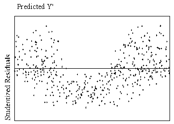
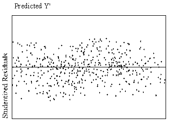
A preferable method of detection is examination of residual plots (plots
of the standardized residuals as a function of standardized predicted values,
readily available in most statistical software). Figure 1 shows scatterplots of residuals that indicate
curvilinear and linear relationships.
| Figure
1.
Example of curvilinear and linear relationships with standardized
residuals by standardized predicted values. |
| Curvilinear Relationship
| Linear Relationship
|
| 
|
The third method of detecting
curvilinearity is to routinely run regression analyses that incorporate
curvilinear components (squared and cubic terms; see Goldfeld and Quandt, 1976
or most regression texts for details on how to do this) or utilizing the
nonlinear regression option available in many statistical packages.
It is important that the nonlinear aspects of the relationship be
accounted for in order to best assess the relationship between variables.
VARIABLES ARE MEASURED WITHOUT ERROR (RELIABLY)
The nature of our educational and social science research means that many
variables we are interested in are also difficult to measure, making measurement
error a particular concern. In
simple correlation and regression, unreliable measurement causes relationships
to be under-estimated increasing the risk of Type II errors.
In the case of multiple regression or partial correlation, effect sizes
of other variables can be over-estimated if the covariate is not reliably
measured, as the full effect of the covariate(s) would not be removed.
This is a significant concern if the goal of research is to accurately
model the “real” relationships evident in the population.
Although most authors assume that reliability estimates (Cronbach alphas)
of .7-.8 are acceptable (e.g., Nunnally, 1978) and Osborne, Christensen, and
Gunter (2001) reported that the average alpha reported in top Educational
Psychology journals was .83, measurement of this quality still contains enough
measurement error to make correction worthwhile, as illustrated below.
Correction for low reliability is
simple, and widely disseminated in most texts on regression, but rarely seen in
the literature. We argue that
authors should correct for low reliability to obtain a more accurate picture of
the “true” relationship in the population, and, in the case of multiple
regression or partial correlation, to avoid over-estimating the effect of
another variable.
Reliability and simple regression
Since “the presence of measurement errors in behavioral research is the
rule rather than the exception” and “reliabilities of many measures used in
the behavioral sciences are, at best, moderate” (Pedhazur, 1997, p. 172); it
is important that researchers be aware of accepted methods of dealing with this
issue. For simple regression,
Equation #1 provides an estimate of the “true” relationship between the IV
and DV in the population:

|
(1) |
In
this equation, r12 is the observed correlation, and r11
and r22 are the reliability estimates of the variables.
Table 1 and Figure 2 presents examples of the results of such a
correction.
|
Table 1: Values of r and r2 after correction for
attenuation
|
|
|
Reliability
of DV and IV
|
|
|
Perfect measurement
|
.80
|
.70
|
.60
|
.50
|
|
Observed r
|
r
|
r2
|
r
|
r2
|
r
|
r2
|
r
|
r2
|
r
|
r2
|
|
.10
|
.10
|
.01
|
.13
|
.02
|
.14
|
.02
|
.17
|
.03
|
.20
|
.04
|
|
.20
|
.20
|
.04
|
.25
|
.06
|
.29
|
.08
|
.33
|
.11
|
.40
|
.16
|
|
.40
|
.40
|
.16
|
.50
|
.25
|
.57
|
.33
|
.67
|
.45
|
.80
|
.64
|
|
.60
|
.60
|
.36
|
.75
|
.57
|
.86
|
.74
|
--
|
--
|
--
|
--
|
|
Note: for simplicity we show an example
where both IV and DV have identical reliability estimates.
In some of these hypothetical examples we would produce impossible
values, and so do not report these.
|
| Figure 2: Change in variance accounted for as correlations are
corrected for low reliability |
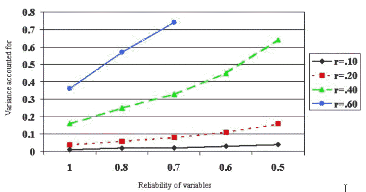 |
As Table 1 illustrates, even in
cases where reliability is .80, correction for attenuation substantially changes
the effect size (increasing variance accounted for by about 50%).
When reliability drops to .70 or below this correction yields a
substantially different picture of the “true” nature of the relationship,
and potentially avoids a Type II error.
Reliability and Multiple Regression
With each independent variable
added to the regression equation, the effects of less than perfect reliability
on the strength of the relationship becomes more complex and the results of the
analysis more questionable. With
the addition of one independent variable with less than perfect reliability each
succeeding variable entered has the opportunity to claim part of the error
variance left over by the unreliable variable(s). The apportionment of the explained variance among the
independent variables will thus be incorrect.
The more independent variables added to the equation with low levels of
reliability the greater the likelihood that the variance accounted for is not
apportioned correctly. This can
lead to erroneous findings and increased potential for Type II errors for the
variables with poor reliability, and Type I errors for the other variables in
the equation. Obviously, this gets
increasingly complex as the number of variables in the equation grows.
A simple example, drawing heavily
from Pedhazur (1997), is a case where one is attempting to assess the
relationship between two variables controlling for a third variable (r12.3).
When one is correcting for low reliability in all three variables
Equation #2 is used:
|

|
(2)
|
Where r11, r22, and r33 are reliabilities, and
r12, r23, and r13 are relationships between
variables. If one is only
correcting for low reliability in the covariate one could use Equation #3:

|
(3)
|
Table 2 presents some examples of corrections for low
reliability in the covariate (only) and in all three variables.
|
Table 2: Values of r12.3 and r212.3
after correction low reliability
|
|
Examples:
|
|
Reliability
of Covariate
|
Reliability
of All Variables
|
|
|
|
|
|
.80
|
.70
|
.60
|
.80
|
.70
|
.60
|
|
r12
|
r13
|
r23
|
Observed r12.3
|
r12.3
|
r12.3
|
r12.3
|
r12.3
|
r12.3
|
r12.3
|
|
.3
|
.3
|
.3
|
.23
|
.21
|
.20
|
.18
|
.27
|
.30
|
.33
|
|
.5
|
.5
|
.5
|
.33
|
.27
|
.22
|
.14
|
.38
|
.42
|
.45
|
|
.7
|
.7
|
.7
|
.41
|
.23
|
.00
|
-.64
|
.47
|
.00
|
--
|
|
.7
|
.3
|
.3
|
.67
|
.66
|
.65
|
.64
|
.85
|
.99
|
--
|
|
.3
|
.5
|
.5
|
.07
|
-.02
|
-.09
|
-.20
|
-.03
|
-.17
|
-.64
|
|
.5
|
.1
|
.7
|
.61
|
.66
|
.74
|
.90
|
--
|
--
|
--
|
|
Note: In some examples we would produce impossible values that we do not
report.
|
Table 2 shows some of the many possible combinations of
reliabilities, correlations, and the effects of correcting for only the
covariate or all variables. Some
points of interest: (a) as in Table
1, even small correlations see substantial effect size (r2) changes
when corrected for low reliability, in this case often toward reduced effect
sizes (b) in some cases the corrected correlation is not only substantially
different in magnitude, but also in direction of the relationship, and (c) as
expected, the most dramatic changes occur when the covariate has a substantial
relationship with the other variables.
ASSUMPTION OF HOMOSCEDASTICITY
Homoscedasticity means that the
variance of errors is the same across all levels of the IV. When the variance of errors differs at different values of
the IV, heteroscedasticity is indicated. According
to Berry and Feldman (1985) and Tabachnick and Fidell (1996) slight
heteroscedasticity has little effect on significance tests; however, when
heteroscedasticity is marked it can lead to serious distortion of findings and
seriously weaken the analysis thus increasing the possibility of a Type I error.
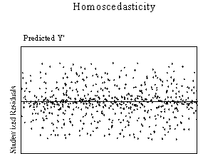
This assumption can be checked by visual examination of a plot of the
standardized residuals (the errors) by the regression standardized predicted
value. Most modern statistical
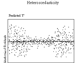
packages include this as an option. Figure
3 show examples of plots that might result from homoscedastic and
heteroscedastic data.
| Figure 3. Examples of homoscedasticity and
heteroscedasticity |
 |
 |
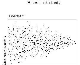 |
Ideally, residuals are randomly scattered around 0 (the horizontal line)
providing a relatively even distribution. Heteroscedasticity
is indicated when the residuals are not evenly scattered around the line.
There are many forms heteroscedasticity can take, such as a bow-tie or
fan shape. When the plot of
residuals appears to deviate substantially from normal, more formal tests for
heteroscedasticity should be performed. Possible
tests for this are the Goldfeld-Quandt test when the error term either decreases
or increases consistently as the value of the DV increases as shown in the fan
shaped plot or the Glejser tests for heteroscedasticity when the error term has
small variances at central observations and larger variance at the extremes of
the observations as in the bowtie shaped plot (Berry & Feldman, 1985).
In cases where skew is present in the IVs, transformation of variables
can reduce the heteroscedasticity.
CONCLUSION
The goal of this article was to
raise awareness of the importance of checking assumptions in simple and multiple
regression. We focused on four
assumptions that were not highly robust to violations, or easily dealt with
through design of the study, that researchers could easily check and deal with,
and that, in our opinion, appear to carry substantial benefits.
We believe that checking these
assumptions carry significant benefits for the researcher. Making sure an
analysis meets the associated assumptions helps avoid Type I and II errors.
Attending to issues such as attenuation due to low reliability,
curvilinearity, and non-normality often boosts effect sizes, usually a desirable
outcome.
Finally, there are many
non-parametric statistical techniques available to researchers when the
assumptions of a parametric statistical technique is not met.
Although these often are somewhat lower in power than parametric
techniques, they provide valuable alternatives, and researchers should be
familiar with them.
References
Berry, W. D.,
& Feldman, S. (1985). Multiple
Regression in Practice. Sage
University Paper Series on Quantitative Applications in the Social Sciences,
series no. 07-050). Newbury Park, CA: Sage.
Cohen, J.,
& Cohen, P. (1983). Applied multiple regression/correlation analysis for the behavioral
sciences. Hillsdale, NJ:
Lawrence Erlbaum Associates, Inc.
Nunnally, J. C. (1978). Psychometric Theory (2nd ed.).
New York: McGraw Hill.
Osborne, J. W., Christensen, W. R., & Gunter, J. (April, 2001).
Educational Psychology from a Statistician’s Perspective:
A Review of the Power and Goodness of Educational Psychology Research.
Paper presented at the national meeting of the American Education
Research Association (AERA), Seattle, WA.
Osborne, J. W. (2001). A new look at outliers and fringeliers: Their effects on statistic accuracy and Type I and Type II error rates.
Unpublished manuscript, Department of Educational Research and Leadership and Counselor Education, North Carolina State University.
Pedhazur, E. J., (1997). Multiple
Regression in Behavioral Research (3rd ed.). Orlando, FL:Harcourt
Brace.
Tabachnick, B. G., Fidell, L. S.
(1996). Using Multivariate
Statistics (3rd ed.). New York:
Harper Collins College Publishers
Tabachnick, B. G., Fidell, L. S.
(2001). Using Multivariate
Statistics (4th ed.). Needham
Heights, MA: Allyn and Bacon
Contact Information:
Jason W. Osborne, Ph.D
ERLCE, Campus Box 7801
Poe Hall 608,
North Carolina
State University
Raleigh NC 27695-7801
(919) 515-1714
Jason_Osborne@ncsu.edu

